Compiler optimization modes
Starting with release 1.17, SambaFlow fully supports two new compiler modes, o0 and o1, that fundamentally change how the compiler prepares your model for execution on the RDU. The biggest difference between the two modes is in how they fuse operators together into basic RDU execution units, called sections.
-
o0 compiles each operator as a seperate section (safe mode).
-
o1 fuses operators. You can control o1 with customizable operator fusion rules and prespecified heuristics.
What is operator fusion? What is a section?
One of the fundamental differences between an RDU and a GPU is that the RDU organizes its compute resources around a dataflow architecture. In a dataflow architecture, the output of one computation can flow to the next (and the next and so on) without wasting a round trip back to memory between every operation. It’s an ideal setup for systems that need pipelines for an immense amount of data, such as machine learning.
To make the best use of our architecture, the compiler has to decide how to lay out these pipelines - in other words, which operators in a model are executed where and when. A single one of our chips, while large, does not have enough compute fabric (PMUs and PCUs) to contain an entire model.
Instead, our compiler divides a model into sections that then serve as the fundamental execution units. Contained within one section is a subgraph of the entire model where a number of operators are fused into one continuous, compound block that executes in its entirely before going back to memory. The term operator fusion comes from the world of GPUs, where multiple discrete operators are fused together into a single compound kernel (see this Medium article). On a GPU, operator fusion is limited in scope and compound kernels are typically written by hand. The RDU, on the other hand, is naturally suited for automatic operator fusion.
How operator fusion relates to compiler modes
There are currently 3 compiler modes: o0, o1, and o3. With each mode, the compiler extends its optimization scope to a wider range:
-
o0 is operator mode, which compiles the model graph with each operator as a seperate section. In other words, it performs no operator fusion at all. o0 is the best option when you first bring up a model for debugging, but performance is not optimal.
-
o1 is module mode, in which the compiler intentionally fuses operators to be in the same section. Operator fusion can be done automatically via an operator fusion rules file or defined manually in your app. o1 enables the best performance, but may require extra customization by you if used with a model that is not supported out of the box.
-
o3 is full graph mode and is the current default. The compiler tries to make all optimization decisions automatically based on the entire graph. o3 achieves better performance than o0, but worse performance than o1 when the model has fusion rules defined.
What is the model graph?
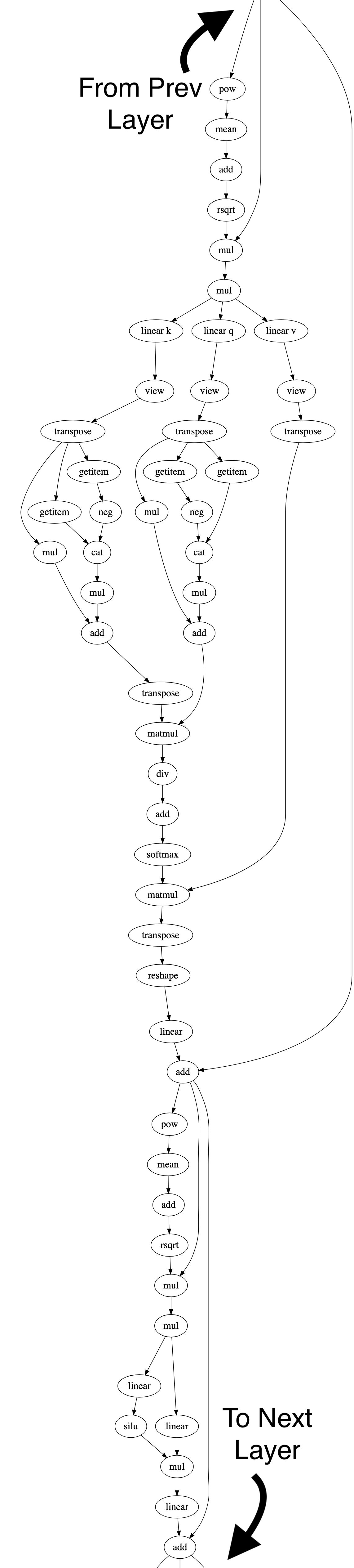
The model graph is a given model’s computation graph. In other words, what you’d get if you took all the operators in a model and connected them together in a big flowchart. Let’s use Llama2 in its 7B parameter configuration, which has 32 encoder layers, as an example.
Each encoder layer in the forward graph contains 51 operators; thus, Llama2 7B inference contains 51*32 = 1632 operators, plus a handful of operators at the beginning and end (to handle the embeddings and loss, etc). The backward graph (used for training) is generated by the compiler using the Autograd algorithm, and has even more operators (the Pytorch documentation includes a discussion of Autograd).
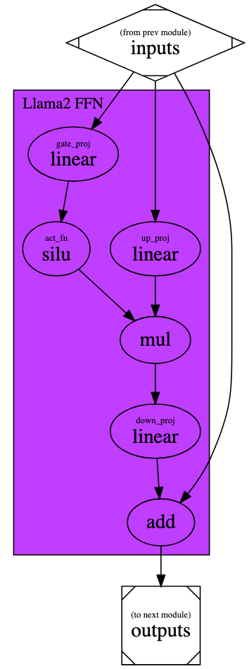
Let’s now look at just one of the modules in the encoder, the Feed Forward Network (FFN). Simplifying some unnecessary details, here’s the PyTorch code for the Llama2 FFN and the computation graph for this FFN:
import torch.nn as nn
from torch.nn.functional import silu
from transformers import AutoConfig

class Llama2FFN(nn.Module):
   def __init__(self, config: AutoConfig) -> None:
      super().__init__()
      self.h_size = config.hidden_size
      self.im_size = config.intermediate_size

      self.gate_proj = nn.Linear(self.h_size, self.im_size, bias=False)
      self.up_proj = nn.Linear(self.h_size, self.im_size, bias=False)
      self.down_proj = nn.Linear(self.im_size, self.h_size, bias=False)

   def forward(self, inputs: torch.Tensor) -> torch.Tensor:
      residual = inputs
      gate_proj_result = self.gate_proj(inputs)
      act_result = silu(gate_proj_result)
      up_proj_result = self.up_proj(inputs)
      down_proj_result = self.down_proj(act_result * up_proj_results)
      outputs = residual + down_proj_result
      return outputs
Compile time differences between o0/o1 and o3
| Models typically compile more slowly with o3 than with o0 or o1 because o3 uses the full graph optimization scope. In contrast, both o0 and o1 have limited optimization scopes and are able to leverage tools in our compiler that fold identical scopes together. That means repeated elements do not have to be processed again and again. |
For example, consider an NLP model with 32 encoders. Each encoder layer has a Multi-Headed Attention (MHA) module, and each of these MHAs has identical sizes and data types. (For details about MHA, this external article is a great explanatory resource.)
With o1, the compiler detects the MHA’s pattern of operators 32 times (once in each encoder layer) and then folds them together into a single operator fusion group. Now, instead of applying optimizations and transformations directly on these operators in-situ on the original graph, the compiler applies them to this folded operator fusion group to essentially do the same thing on all 32 instances of the operator pattern at once.
Operator fusion example
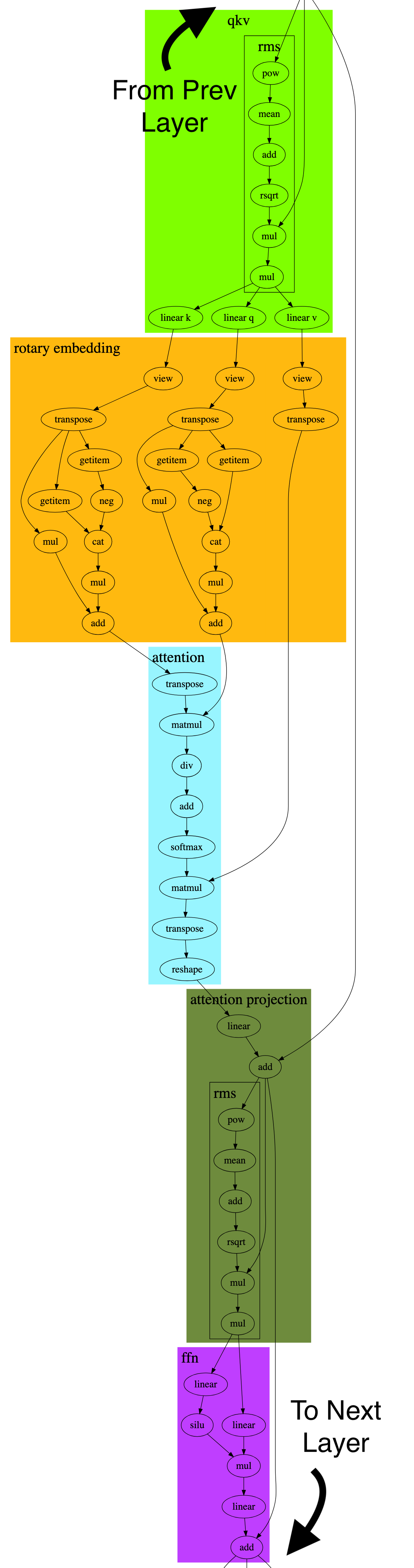
The following diagram shows an example of operator fusion on LLaMA2 7B. The graph on the left represents a snippet of Llama2’s compute graph, showing just one encoder layer. (weights are not shown; only the operations.) The full graph has many such layers (e.g. 32 layers for Llama 7B) and thousands of operators. Meanwhile, the graph on the right shows how the compiler fuses these operators in o1 mode.
|
|
|
How do you use o0 and o1?
To use o0, just add -o0 to your compile command.
To use o1, you have two choices: automatic fusion or manual fusion.
Automatic fusion
To use automatic fusion, add -o1 --optimization-rules PATH/TO/YOUR/RULES/FILE.yaml to your compile command. You do not need to make any modifications to your app or your model. The operator fusion rules file matches particular patterns of operators in the graph and then fuses them into sections. Currently, we have fusion rules files defined for many different NLP models available in sambaflow/o1_optimizations/opfusion_rules/. For details about defining your own patterns, see Operator fusion rule yaml syntax.
If you don’t specify an operator fusion rule with --optimization-rules, then o1 behaves like o0.
|
Manual fusion
Manual fusion is done by tagging PyTorch modules in your model with a Python decorator. Here’s an example:
from sambaflow.samba.directives import op_fusion
from sambaflow.o1_optimizations.modules.opfusionheuristics import OpFusionHeuristics

@op_fusion(func_name="my_fused_attn_proj", heuristic=OpFusionHeuristics.SAFE_GEMM)
class AttentionProjection(nn.Module):
    def __init__(self, args: ModelArgs):
       ...
The func_name can be whatever you want as long as each op_fusion has a unique name. The heuristic is optional, but recommended where possible. For details, see Operator fusion heuristics.
With manual fusion, the optimal fusion groupings for runtime performance may not align with your modules as-is, and thus you may need to move some operators around to adjacent (or new) modules. A detailed guide on optimizing a model to achieve the best performance on RDU is currently in progress.
Operator fusion heuristics
Tagging an operator fusion rule with a heuristic lets the compiler know it should use a specific strategy for optimizing this module. Our heuristics are plug-and-play and can be used to optimize any module that meets each heuristic’s constraints. The trade-off is that each heuristic can be applied only to certain types of modules; see Supported heuristics. If no heuristic is specified for a module, the compiler applies general optimizations to that portion of the compute graph, akin to what it would do in o3 mode.
Each heuristic is a full package of optimizations, including tiling, sharding, internal section-cuts, and par factors, and, if applicable, even co-optimizes both the forward sections and the autograd-generated backward sections.
The optimizations performed by o3 are done using generic algorithms that need to be able to handle any sort of graph fed into it. In contrast, operator fusion heuristics use specific algorithms that are especially well suited to particular kinds of modules. By way of analogy, think of the optimizations done by o3 as akin to buying a suit off the racks at a department store, while the optimizations done by the operator fusion heuristics are more like going to a fine tailor and being fitted for a custom suit.
How do I use heuristics?
Heuristics can be used with both automatic fusion rules and manual fusion rules. For an example with manual fusion rules, see Manual fusion above. For automatic fusion with a fusion rule, you can specify a heuristic label like this:
example_pattern:
    heuristic: SAFE_GEMM
    pattern:
        linear_a:
           op_type: linear
           ...
Supported heuristics
Currently, supported heuristics include GEMM heuristic variations, the MHA heuristic, and the SDPA heuristic.
GEMM heuristic variations
The GEMM heuristic is a collection of heuristics that share common logic. They’re applicable to hyperfunctions that are dominated by a single large matrix multiply (GEMM) operation. (e.g. linear, addmm, or matmul operators). NLP applications typically have multiple modules that fit this description.
The following variations are available:
-
DEFAULT_GEMM, SAFE_GEMM, AGGRESSIVE_GEMM
These three variations each maximize the throughput through a GEMM-dominated hyperfunction. The difference between them is how they do PCU/PMU resource estimation. Because optimization happens before the final PEF is generated, each heuristic must estimate how many PCUs and PMUs certain combinations of optimizations translate to in the PEF file. If the heuristic requests more resources than are available in a section, then compilation fail in a later compiler layer.
-
DEFAULT uses the default estimations. These estimations generally work and are always being improved, but they’re not perfect.
-
SAFE tries to be careful with resource estimates and always works. It might shard to a lower degree and always puts a GEMM in its own section without any other nodes. Both of these things will hurt performance.
-
AGGRESSIVE tries to push certain optimizations as far as they can go, but has a higher risk of failing compilation.
-
-
INFERENCE_GEMM, SAFE_INFERENCE_GEMM
These two variations are for cached inference.
-
INFERENCE_GEMM is more aggressive when trying to fit more GEMMs into a single section at the expense of fewer shards and lower par factors compared to DEFAULT_GEMM. Flag sections that are dominated by memory latency rather than compute latency with INFERENCE_GEMM.
-
SAFE_INFERENCE_GEMM, is like SAFE_GEMM. It sacrifices performance to ensure that the compilation completes and a PEF is successfully generated.
-
MHA heuristic and SDPA heuristic
The MHA (Multi-headed attention) heuristic is for any multi-headed attention block for models that have 2 matmul operators with a softmax operator between them. It’s fine if the module contains other operators, as long as they are not GEMMs.
The SDPA (scaled dot product attention) heuristic has similar optimization logic and parameters, but is specifically for a rolled up scaled dot product attention PyTorch operator. See this external link for details.
Learn more!
-
See SambaFlow compiler overview for an introduction to how the compiler works.
-
See Operator fusion rule yaml syntax for a reference to the operator fusion rule yaml syntax.
-
See Compiler argument reference for a reference to supported compiler arguments.