Compilation, training, and inference

This tutorial takes you a few steps beyond our Hello SambaFlow! tutorial: You also learn about dataset preparation, testing (validation), and inference. The result is a complete end-to-end machine learning workflow:

Check the SambaFlow installation.
Prepare the dataset.
Compile the model.
Train the model.
Test (validate) the model.
Run inference on the model and visually check predictions.

You’ll download the tutorial files from our public GitHub repo and the data files (the MNIST datasets) from the internet.

We discuss the code for this model in Examine LeNet model code.

Prepare your environment

To prepare your environment, you:

Check your SambaFlow installation.
Download the tutorial files from GitHub.
Download the data files from the internet.

Check your SambaFlow installation

You must have the sambaflow package installed to run this example and any of the tutorial examples.

To check if the package is installed, run this command:
- For Ubuntu Linux
  $ dpkg -s sambaflow
- For Red Hat Enterprise Linux
  $ rpm -qi sambaflow
Examine the output and verify that the SambaFlow version that you are running matches the documentation you are using.
If you see a message that sambaflow is not installed, contact your system administrator.

Download the model code from GitHub

Before you start, clone the SambaNova/tutorials GitHub repository, as instructed in the README.

In the following command-line examples we assume that you cloned the repository into your home directory and that created the ~/tutorials directory.

After a SambaFlow upgrade, you might have to clone the repository again if your model no longer works.

The LeNet tutorial includes the following files:

lenet.py. Code for compiling the model for training, running initial training, running training from a checkpoint, and running inference.
visualize_predictions.ipynb. A Jupyter notebook file that visualizes the results of inference.
mnist_utils.py file, which includes
- A CustomMNIST class that you will use to create a dataset from Fashion MNIST.
- A write_labels() function for writing labels in the MNIST-compatible format.

Prepare the dataset

In contrast to the classic MNIST dataset, which consists of hand-written digits, Fashion MNIST uses images from Zalando a fast-fashion online retailer.

60,000 images in the training set
10,000 images in the test set.

We decided to use Fashion MNIST in this tutorial because it’s a little more challenging to train than the original MNIST dataset and you can actually examine the output of the inference run.

Create a subdirectory for your datasets in your home directory. In this example we use $HOME/datasets.
```
$ mkdir -p $HOME/datasets/
```
Create the subdirectory for the Fashion MNIST dataset and set the DATADIR environment variable to point to this location.
```
$ mkdir -p $HOME/datasets/fashion-mnist
$ export DATADIR=$HOME/datasets/fashion-mnist
```

Download and extract the datasets.

$ wget -P $DATADIR http://fashion-mnist.s3-website.eu-central-1.amazonaws.com/train-images-idx3-ubyte.gz
$ wget -P $DATADIR http://fashion-mnist.s3-website.eu-central-1.amazonaws.com/train-labels-idx1-ubyte.gz
$ wget -P $DATADIR http://fashion-mnist.s3-website.eu-central-1.amazonaws.com/t10k-images-idx3-ubyte.gz
$ wget -P $DATADIR http://fashion-mnist.s3-website.eu-central-1.amazonaws.com/t10k-labels-idx1-ubyte.gz
$ cd $DATADIR
$ gunzip *gz

Compile the model

Before you can train a model to run on RDU, you have to compile for training.

Each model’s code contains a compilation function. You call the function as python <model.py> compile <compile_args>. See the Compiler Reference for some background on compiler arguments.

How to compile the model

Change to the model directory:
```
$ cd ~/tutorials/lenet
```
Compile the model
```
$ python lenet.py compile --batch-size 32 \
  --pef-name lenet-b32
```
Compilation messages are sent to stdout. You can ignore most messages. At the end of that output you will see the following message:
```
[info   ] PEF file /home/snuser1/tutorials/lenet/out/lenet-b32/lenet-b32.pef created
```
You’ll need this PEF file to run training, testing, and inference.

Compilation arguments

Before calling the compile command have a look at available compilation arguments.

All models support the shared arguments that documented in the Compiler Reference.
All models support an additional set of experimental shared arguments, usually used with working with SambaNova Support. To include these arguments in the help output, run <model_name>.py compile --debug --help.
Each model has an additional set of model-specific arguments. Those arguments are different for different models.

To get a list of possible arguments call:

$ python lenet.py compile --help

If you run the compile command without parameters, the compiler uses a set of reasonable defaults.

The Compiler Reference discusses arguments used by all models. Here’s a list of other arguments:

--num-classes. Defines the number of classes used for classification. In this example you use the MNIST dataset to recognize handwritten digits from 0 to 9, so the number of classes is 10. This is the value that is set in the application’s code.

--num-features. Defines the number of pixels for each image in the dataset. With the Fashion MNIST dataset we use in this tutorial, each picture is 28×28 pixels, so num-features is 784. This is the value that is set in the application’s code.

--batch-size. See batch-size.

--output-folder. Output folder where compilation artifacts will be stored. By default, the compiler creates a folder called out in your current folder. Inside that directory the compilation script creates a separate directory for each compilation run.

--pef-name — See pef-name.

Train the model

SambaFlow supports a run command for training, testing, and inference.

Common arguments to run

You can check the available command-line options by using --help:

$ python lenet.py run --help

Many run arguments are predefined by SambaFlow, but most models also define model-specific arguments. The most important arguments for this tutorial are:

--pef. Full path for a PEF file that was generated by the compiler. Copy-paste the filename from the last line of the compilation output.
--data-dir. Data directory. In this tutorial, the directory to which you downloaded the MNIST dataset.
--ckpt-dir. During training, SambaFlow saves checkpoints to this directory. You can later load a checkpoint to continue a training run that was interrupted, or load a checkpoint for inference.
--init-ckpt-path. Full path for a checkpoint file. Use this file path to continue training if you stopped.

Train for one epoch

Start a training run for one epoch using:

The dataset you downloaded before.

The PEF file you generated in the compilation step.

$ export DATADIR=$HOME/datasets
$ python lenet.py run \
    --batch-size 32 \
    --pef out/lenet-b32/lenet-b32.pef \
    --data-dir $DATADIR \
    --ckpt-dir checkpoints

With this model and dataset, training should not take more than a minute. On stdout, you see a training log, which includes accuracy and loss. Here’s an example, abbreviated in the middle.

Using dataset: /home/snuser1/datasets/fashion-mnist/train
==============================
Initial epoch:   0, initial step:      0
Target epoch:    1, target step:    1875
Epoch [1/1], Step [100/1875], Loss: 1.5596
Epoch [1/1], Step [200/1875], Loss: 1.2914
Epoch [1/1], Step [300/1875], Loss: 1.1413
Epoch [1/1], Step [400/1875], Loss: 1.0423
...
Epoch [1/1], Step [1400/1875], Loss: 0.7138
Epoch [1/1], Step [1500/1875], Loss: 0.7010
Epoch [1/1], Step [1600/1875], Loss: 0.6893
Epoch [1/1], Step [1700/1875], Loss: 0.6792
Epoch [1/1], Step [1800/1875], Loss: 0.6695

Verify that the model saved a checkpoint file under ./checkpoints. The file name corresponds to the number of training steps taken.
```
$ ls  ./checkpoints/
```

Train for two and more epochs using the checkpoint

You can continue training from the checkpoint that was saved during the first training run. For more complex models, multiple training runs that progressively train from a checkpoint are helpful. If you train for several epochs and each epoch takes significant time (hours or days):

Stop training after several epochs.
Start training again when you’re ready and pass in the last saved checkpoint.

Using checkpoints is also helpful when you experience an interrupt in the training run for some reason (e.g. hardware or software failure). Just start training from the last checkpoint!

To start training from a saved checkpoint, specify the checkpoint file with the --init-ckpt-path argument and specify the total number of epochs to train for with --num-epochs. In this example we train for two total epochs. The checkpoint was saved after one epoch, so this second training run will be for one more epoch.

For the second training run, run this command:

$ python lenet.py run \
    --batch-size 32 \
    --pef out/lenet-b32/lenet-b32.pef \
    --data-dir $DATADIR \
    --ckpt-dir checkpoints \
    --init-ckpt-path checkpoints/1875.pt \
    --num-epochs 2

This time the training run started from 1875 steps and reached 3750 steps.

Examine the output, which shows that the loss goes down and the accuracy increases a bit. Here’s an example, abbreviated in the middle.

Using dataset: /home/snuser1/datasets/fashion-mnist/train
==============================
Initial epoch:   1, initial step:   1875
Target epoch:    2, target step:    3750
Epoch [2/2], Step [1975/3750], Loss: 0.4920
Epoch [2/2], Step [2075/3750], Loss: 0.4945
Epoch [2/2], Step [2175/3750], Loss: 0.4875
Epoch [2/2], Step [2275/3750], Loss: 0.4927
...
Epoch [2/2], Step [3275/3750], Loss: 0.4761
Epoch [2/2], Step [3375/3750], Loss: 0.4745
Epoch [2/2], Step [3475/3750], Loss: 0.4729
Epoch [2/2], Step [3575/3750], Loss: 0.4720
Epoch [2/2], Step [3675/3750], Loss: 0.4707

Verify that the resulting checkpoint is saved under ./checkpoints/ as 3750.pt.
```
$ ls checkpoints/
3750.pt  1875.pt
```

Optionally, use the new checkpoint to train for the third and other epochs by changing the number of epochs and the checkpoint file name. For example:

$ python lenet.py run \
    --batch-size 32 \
    --pef out/lenet-b32/lenet-b32.pef \
    --data-dir $DATADIR \
    --ckpt-dir checkpoints \
    --init-ckpt-path checkpoints/3750.pt \
    --num-epochs 3

Verify that the loss decreases and the accuracy increases—but only by just a notch. For this simple model we can stop training after 2-3 epochs. For more complex models and datasets, the number of epochs you need for optimal accuracy is different.

Test model accuracy

After you trained the model for several epochs, you can test its accuracy.

Pick one of the saved checkpoints and run a test against the test dataset.

$ python lenet.py run --test \
    --batch-size 32 \
    --pef out/lenet-b32/lenet-b32.pef \
    --data-dir $DATADIR \
    --init-ckpt-path checkpoints/1875.pt

Verify that your output looks like this (your exact numbers might be different):

Using dataset: /home/snuser1/datasets/fashion-mnist/t10k
Test Accuracy: 82.57  Loss: 0.5030

To compare the accuracy for different number of epochs, run the same command with different checkpoint filenames and compare the accuracy and loss numbers. If the accuracy is still steadily increasing and the loss is decreasing, then running the model for more epochs will likely increase accuracy.
Run the model for more epochs if you expect benefits.

Run and verify inference

When you are satisfied with the accuracy you can use the model for inference. Inference means that you use a file with the same data format but without labels. The inference run adds the labels.

For large models, the workflow includes a separate compilation step for inference. For simple models, that step isn’t necessary. We can use the PEF file we generated during the initial compilation.

Run inference

To run inference:

Create a new file with images but no labels from the test dataset.

$ cp $DATADIR/t10k-images-idx3-ubyte $DATADIR/inference-images-idx3-ubyte

Run inference for this new dataset. You pass in both the PEF and the checkpoint file.

$ python lenet.py run --inference \
    --batch-size 32 \
    --pef out/lenet-b32/lenet-b32.pef \
    --data-dir $DATADIR \
    --dataset-name inference \
    --results-dir ./results \
    --init-ckpt-path checkpoints/3750.pt

The command generates a list of predictions and stores it in the same format as the labels file.

To verify that the predictions file has been created, go to the results directory.
```
$ ls -l ./results
```
Look for a recently created file named similar to MNIST label files. For example:
```
-rw-rw-r--. 1 snuser1 snuser1 10008 Jul  6 13:04 prediction-labels-idx1-ubyte
```

Check predictions

To check predictions, it’s easiest to look at the images that were used for inference and at the generated prediction (labels). Then we can estimate the prediction accuracy visually.

Check that Jupyter Notebook is running on the RDU host by running the following command:
```
$ cd ~/tutorials/lenet
$ nohup jupyter-notebook --ip=0.0.0.0 --no-browser &
```
Enter the Jupyter URL in a browser that has access to the RDU host. You will see a list of files including visualize_predictions.ipynb.
Open visualize_predictions.ipynb. You should see something like this.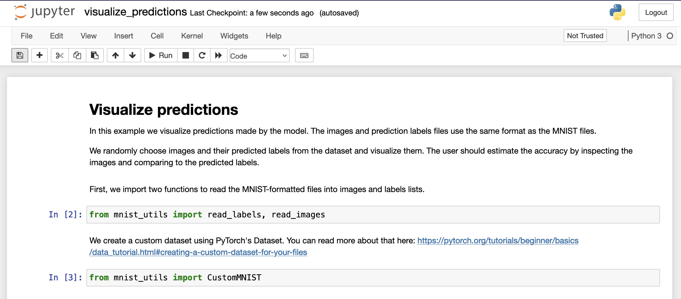
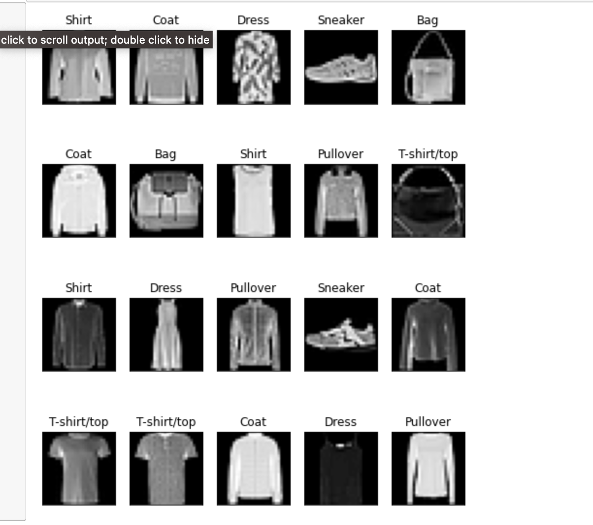
Run the notebook cell by cell (or all cells altogether). At the bottom you will see the predictions which look like this:
Try to estimate visually how many of the images the model got right and wrong.

Learn more!

See Examine LeNet model code for a discussion of the code.
See Model conversion overview if your goal is to port a model. That document points to a tutorial that examines a ported model.