Architecture and workflows
SambaFlow™ is a software stack that is running on DataScale® hardware.
At the bottom, we have the SambaNova Reconfigurable Dataflow Unit™ and the DataScale hardware.
-
SambaNova Reconfigurable Dataflow Unit is a processor that provide native dataflow processing and programmable acceleration. It has a tiled architecture that consists of a network of reconfigurable functional units. The architecture enables a broad set of highly parallelizable patterns contained within dataflow graphs to be efficiently programmed as a combination of compute, memory and communication networks.
-
SambaNova Systems DataScale is a complete, rack-level, data-center-ready accelerated computing system. Each DataScale system configuration consists of one or more DataScale nodes, integrated networking and management infrastructure in a standards-compliant data center rack.
The SambaFlow stack automatically extracts, optimizes and maps dataflow graphs onto RDUs, supporting high performance without the need for low-level kernel tuning. The stack consists of these components:
-
SambaNova Runtime. Allows system administrators to perform low-level management tasks. SambaNova Runtime talks directly to the hardware and includes the SambaNova daemon and some configuration tools.
-
SambaFlow Python SDK. A custom version of PyTorch that enables developers to create and run models on SambaNova hardware.
-
SambaFlow models. Models that are included in your SambaNova environment at
/opt/sambaflow/apps/.
Developers can control SambaFlow behavior at different levels of the stack, for example, by specifying compiler flags or using the Python SDK.
SambaFlow example applications (in /opt/sambaflow/apps/starters) allow you to examine the Python code and then perform compile and training runs.
| SambaNova is in the process of determining which of the models are fully supported, and which are considered primarily examples for exploration. |
This topic looks at the components of SambaFlow and explains what matters to developers.
| For an in-depth discussion, see our white paper SambaNova Accelerated Computing with a Reconfigurable Dataflow Architecture |
Architecture
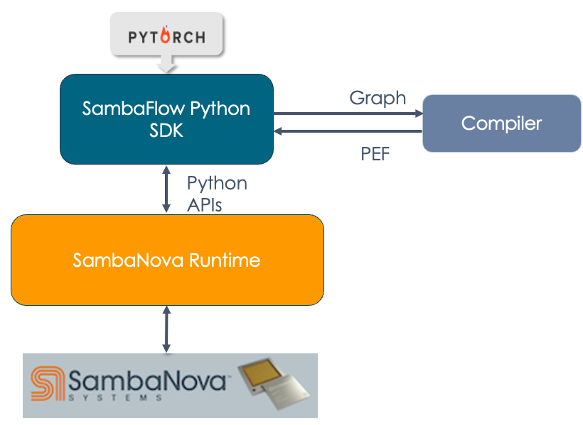
The following image shows the hierarchy of SambaFlow components and how different components interact with each other.
-
DataScale. At the bottom of the stack is the SambaNova DataScale® hardware.
-
SambaNova Runtime. At the next level is the SambaNova Runtime component. This component allows system administrators to perform configuration, fault management, troubleshooting, etc. See the SambaNova Runtime documentation for details.
-
SambaFlow Python SDK. Most developers use the SambaFlow Python SDK to compile and run their models on SambaNova hardware.
-
The developer writes the model code using the Python SDK. This document includes several examples.
-
The developer compiles the model.
-
The compiler returns a PEF file.
-
The developer trains the model by passing in the PEF file and the training dataset. Training happens on hardware.
-
Finally, the developer can use the trained model with a test dataset to verify the model, or run inference using the model. See the SambaFlow API Reference
 .
.
-
Recommended workflow
Here’s the recommended workflow.
Compile
A SambaNova system can reconfigure the hardware to perform accelerated computation and data movement that is specific for a model. When SambaFlow compiles a model, it generates a dataflow graph, which is similar to a PyTorch computational graph. To run the model, that graph must be traced before it can be placed onto the RDU. The compiler generates a PEF file that encapsulates those instructions. You can submit the PEF file when you do training and inference runs.
When you compile a model, specify the location of the PEF file that the compiler will generate as part of the compile command.
Each model has different command-line arguments. You can use --help to see the arguments.
|
Test run
After compilation you can do a test run of the compiled model and check if it runs correctly on the hardware and software combination.
During this step:
-
You include the PEF file that was generated by the compiler in the
compilecommand. The command uploads the PEF file to the node. -
The system configures all necessary elements (PCU and PMU) and creates links between them using on-chip switches.
A test run is not mandatory, but it’s recommended to test the model before starting a long run with many epochs.
The top-level help menu for many models shows a test command. In contrast to run --test, the test command is used primarily internally to compare results on CPU and results on RDU.
|
Training run
During the training run, you feed data to the compiled model. The training run lasts the number of epochs that you specify on the command line. Other command-line options also affect the training. Each time a training run completes, a checkpoint is saved to the /checkpoints directory.
During training, information about accuracy and loss are sent to stdout. When accuracy looks good enough, you can validate against the test dataset. If necessary you can continue training. If everything looks good, you can use the last checkpoint for inference.
Inference run
When the results of validation look good, you can run inference. You pass in the PEF and a checkpoint and a dataset to have the model do actual work. For example, in one tutorial in this doc set, we pass in the unlabeled dataset that’s part of the Fashion MNIST dataset, run inference, and then visually examine the labels that our model assigned.